Urban Pulse: Decoding NYC’s Taxi Tapestry - Analyzing Tip Amounts and Drop Off Distance

Project description: Embark on a data journey through the bustling streets of New York City with my EDA project for the New York City Taxi and Limousine Commission (NYC TLC). In this project I uncover the secrets of taxi ridership and visualize the pulse of the city through EDA and data visualization work. Including data structuring and cleaning, as well as any matplotlib/seaborn and tableau visualizations created to help understand the data.

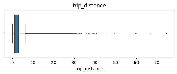
1. Boxplots

Perform a check for outliers on relevant columns such as trip distance and trip duration.

# Create box plot of trip_distance
plt.figure(figsize=(7,2))
plt.title('trip_distance')
sns.boxplot(data=None, x=df['trip_distance'], fliersize=1)

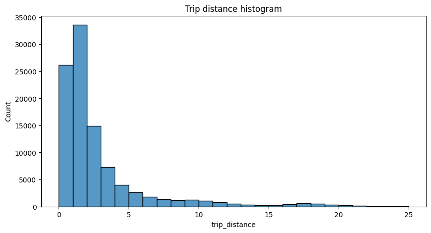
# Create histogram of trip_distance
plt.figure(figsize=(10,5))
sns.histplot(df['trip_distance'], bins=range(0,26,1))
plt.title('Trip distance histogram')

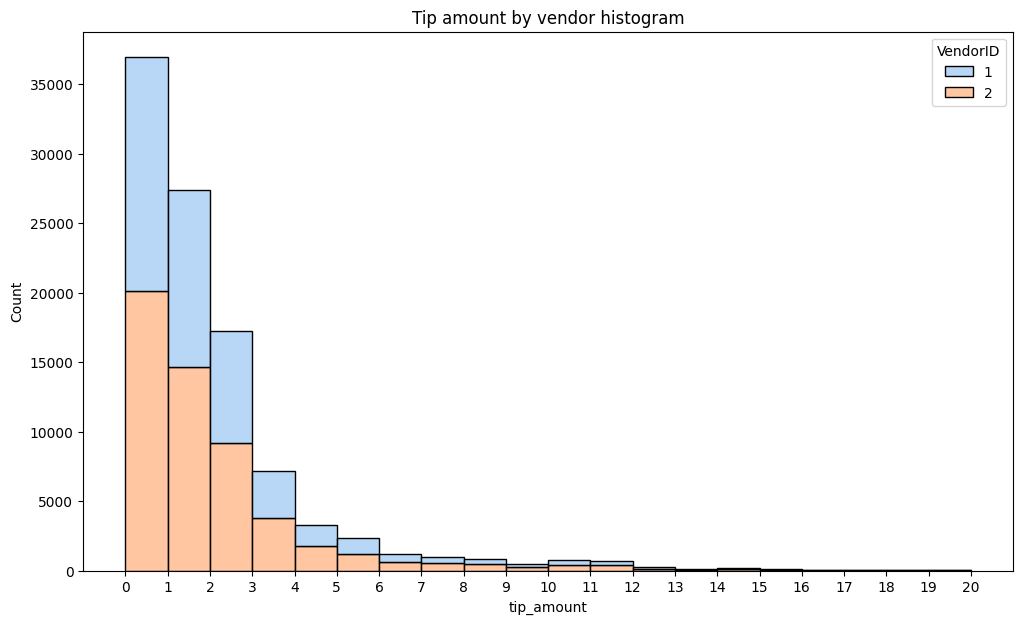
Separating the tip amount by vendor reveals that there are no noticeable aberrations in the distribution of tips between the two vendors in the dataset. Vendor two has a slightly higher share of the rides, and this proportion is approximately maintained for all tip amounts.

# Create histogram of tip_amount by vendor
plt.figure(figsize=(12,7))
ax = sns.histplot(data=df, x='tip_amount', bins=range(0,21,1), 
                  hue='VendorID', 
                  multiple='stack',
                  palette='pastel')
ax.set_xticks(range(0,21,1))
ax.set_xticklabels(range(0,21,1))
plt.title('Tip amount by vendor histogram')

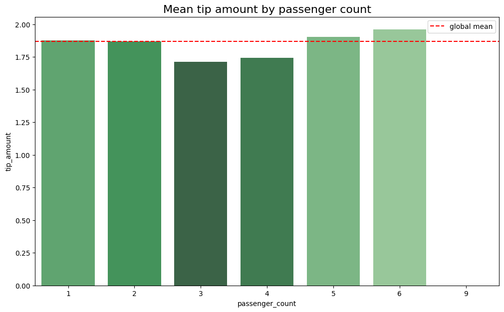
Tip amounts show minimal variation based on passenger count. While there’s a noticeable dip for four-passenger rides, this is anticipated due to the lower frequency of such rides in the dataset, second only to rides with zero passengers.

# Create bar plot for mean tips by passenger count
data = mean_tips_by_passenger_count.tail(-1)
pal = sns.color_palette("Greens_d", len(data))
rank = data['tip_amount'].argsort().argsort()
plt.figure(figsize=(12,7))
ax = sns.barplot(x=data.index,
            y=data['tip_amount'],
            palette=np.array(pal[::-1])[rank])
ax.axhline(df['tip_amount'].mean(), ls='--', color='red', label='global mean')
ax.legend()
plt.title('Mean tip amount by passenger count', fontsize=16)

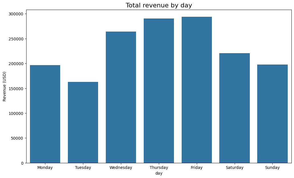
Unexpectedly, Wednesday to Saturday recorded the highest daily ride numbers, with Sunday and Monday having the fewest.

# Create bar plot for ride count by day
plt.figure(figsize=(12,7))
ax = sns.barplot(x=daily_rides.index, y=daily_rides)
ax.set_xticklabels(day_order)
ax.set_ylabel('Count')
plt.title('Ride count by day', fontsize=16)

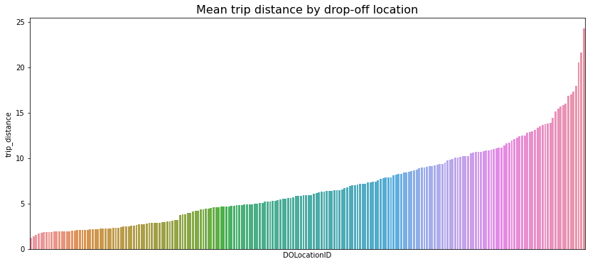
2. Plot mean trip distance by drop-off location

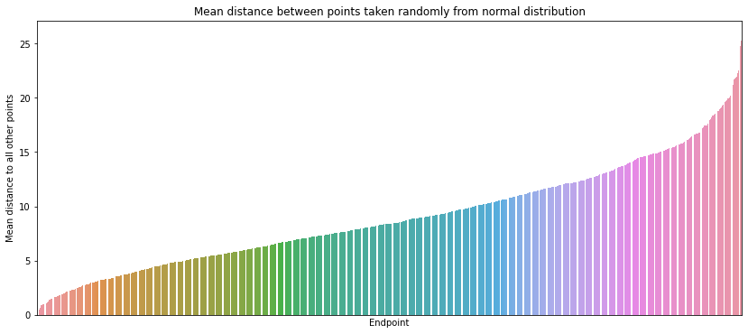
This graph shows a curve akin to the cumulative density function of a normal distribution. In simple terms, it suggests that drop-off points are evenly spread across the area. This is valuable information since the dataset lacks geographic coordinates, making it challenging to assess location distribution.

df['DOLocationID'].nunique()
distance_by_dropoff = df.groupby('DOLocationID')[['trip_distance']].mean()

distance_by_dropoff = distance_by_dropoff.sort_values(by='trip_distance')
distance_by_dropoff
plt.figure(figsize=(14,6))
ax = sns.barplot(x=distance_by_dropoff.index, 
                 y=distance_by_dropoff['trip_distance'],
                 order=distance_by_dropoff.index)
ax.set_xticklabels([])
ax.set_xticks([])
plt.title('Mean trip distance by drop-off location', fontsize=16);
test = np.round(np.random.normal(10, 5, (3000, 2)), 1)
midway = int(len(test)/2)  
start = test[:midway]      
end = test[midway:]       

distances = (start - end)**2           
distances = distances.sum(axis=-1)
distances = np.sqrt(distances)

test_df = pd.DataFrame({'start': [tuple(x) for x in start.tolist()],
                   'end': [tuple(x) for x in end.tolist()],
                   'distance': distances})
data = test_df[['end', 'distance']].groupby('end').mean()
data = data.sort_values(by='distance')
data.reset_index(inplace=True)  

plt.figure(figsize=(14,6))
ax = sns.barplot(x=data.index,
                 y=data['distance'],
                 order=data.index)
ax.set_xticklabels([])
ax.set_xticks([])
ax.set_xlabel('Endpoint')
ax.set_ylabel('Mean distance to all other points')
ax.set_title('Mean distance between points taken randomly from normal distribution');

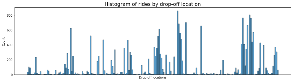
3. Histogram of rides by drop-off location

Note that among the 200+ drop-off locations, a small set attracts the majority of traffic, while the rest receive fewer trips. It’s probable that these high-traffic spots are close to popular tourist attractions like the Empire State Building or Times Square, airports, and transit hubs. Unfortunately, the data lacks information on the specific location corresponding to each ID, which would have been quite useful.

# Check if all drop-off locations are consecutively numbered
df['DOLocationID'].max() - len(set(df['DOLocationID']))
plt.figure(figsize=(16,4))
# DOLocationID column is numeric, so sort in ascending order
sorted_dropoffs = df['DOLocationID'].sort_values()
# Convert to string
sorted_dropoffs = sorted_dropoffs.astype('str')
# Plot
sns.histplot(sorted_dropoffs, bins=range(0, df['DOLocationID'].max()+1, 1))
plt.xticks([])
plt.xlabel('Drop-off locations')
plt.title('Histogram of rides by drop-off location', fontsize=16);